지난 포스트에서는 파이썬으로 인공신경망과 역전파 등을 포함해 MLP를 구현해 보았다. 이번에는 자연어 처리에서 많이 쓰였던 RNN신경망을 구현해보고자 한다. (요즘에는 트랜스포머가 모든 걸 그냥 씹어먹는 경향이 있지만 시계열 데이터는 대부분 RNN계열 모델을 많이 쓰는 편이다.) 코드 중 일부는 지난 포스트에 미리 짜 놓은 함수와 클래스를 일부 사용할 예정이다.
파이썬으로 기초 MLP 구현하기
이번에는 기억을 되살려 tensorflow, pytorch를 사용하지 않고 파이썬만을 사용하여 Multi Layer Perceptron(MLP)를 구현해보도록 하겠다. 구현할 함수는 딱 4개밖에 없다. 구현할 것들 backpropagation 역전파 Me..
hi-lu.tistory.com
0. 시작하면서
RNN은 Recurrent Neural Network로, 순환 신경망을 의미한다. 주로 이 모델을 사용하는 경우는 시계열 데이터를 다룰 때다. 이후 시계열 데이터를 input으로 넣으면 과거 데이터가 희석되는 경향과 gradient vanishing 현상으로 인해 LSTM, GRU 등이 나타나기도 했다. (실제로 RNN보다는 LSTM이 더 많이 쓰인다.) 대표적인 시계열 데이터는 자연어가 있다.
참고로 자연어를 어떻게 인공신경망에 넣는지 간단히 설명하자면 아래와 같다.
- ['나는', '사과를' ,'먹는다.'] 라는 문장을 넣고 싶다. 이 친구를 임베딩 해서 벡터로 만들어준다.
- [[12], [23], [45]] 대충 이런 벡터로 표현했다고 하자. 벡터니까 이제 인공신경망에 넣을 수 있다.
- [[99], [96], [39]] 그래서 이런 벡터를 인공신경망이 output으로 뱉었다고 하자. 이를 디코딩해서 우리가 알아볼 수 있는 문자로 치환한다.
- ['I', 'ate', 'apple']이 되었다!
이해를 돕기 위해 자연어 번역 예제를 간단히 가공해보았다. 이제 이 인공신경망을 파이썬과 numpy 라이브러리로 짜 보도록 하자.
1. 주의할 점
입력의 차원
MLP를 짤 때에는 (batch_size, feature 수)로 input의 shape가 간단했다. 하지만 RNN은 시계열 데이터를 input으로 받는다. 이때 input의 shape는 (batch_size, 시계열 timestamp, embedding 차원)가 된다. 위의 '나는 사과를 먹는다'를 예시로 들자면 문장이 하나(1), 시계열 수는 단어 수인 셋(3), 임베딩 차원은 1이므로 (1,3,1)이 되는 것이다. 참고로 tensorflow나 torch에서는 batch_size와 timestamp의 위치가 달라지기도 한다. 하지만 이번 구현에서는 (batch_size, timestamp, embedding)의 순서로 input이 들어온다 가정하자.
RNN의 구조
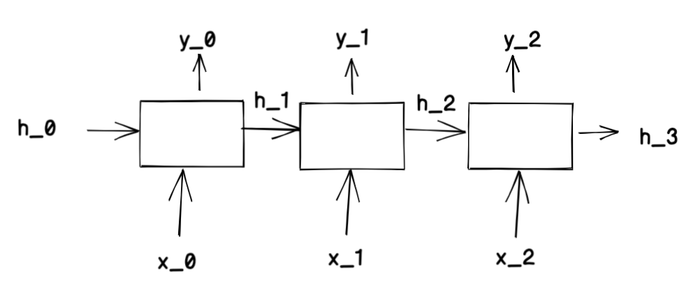
RNN은 hidden_state와 x를 input으로 받는 구조이다.
RNN(x_t, h_t)
우리는 지난 포스트에서 신경망의 기본 구조는 x * weight + bias인 것을 확인했다. RNN도 똑같다. input인 x[t]와 h에 대해서도 같은 연산을 해주면 된다.
[x[t] * weight_x , h_t * weight_h] + bias
결국 weight의 입력 차원은 MLP에서의 weight보다 2배가 되는 것으로, 코드로 나타내면 가중치 weight[t]는 다음과 같다.
self.in_size = self.embedding_size
w_h = np.random.rand(hidden_dim, hidden_dim)
w_x = np.random.rand(self.in_size, hidden_dim)

weight = np.concatenate((w_h, w_x), axis= 0) #(self.in_size+hidden_dim , hidden_dim)
이 시계열 t일 때의 output (y_t, h_(t+1)) 중 h_(t+1)은 다음 timestamp의 input h로 들어가게 된다.
여기서 RNN layer 3개를 더 얹은 Deep RNN 구조를 보자.
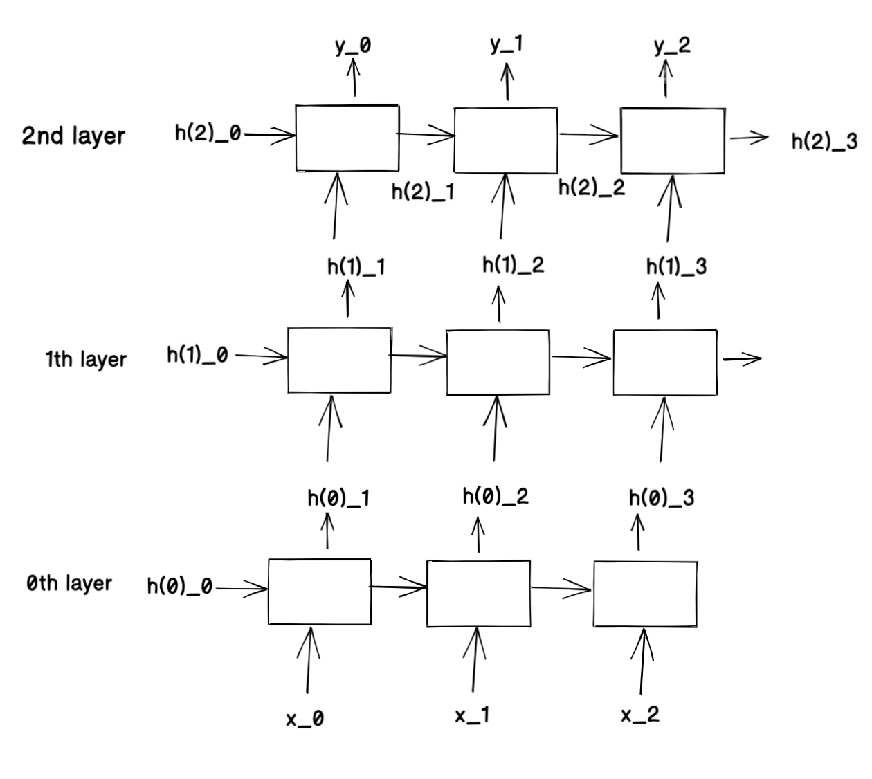
이 구조를 위해 달라질 것은 self.in_size에 들어갈 값이 x의 크기가 아닌 h(i-1)의 크기가 된다는 것이다.
2. 구현
Tanh
순환신경망은 활성화 함수로 주로 tanh를 사용하는데, 수식은 아래와 같다.
tanh(x) = (exp(x) - exp(-x)) / (exp(x) + exp(-x))
이를 함수로 나타내면 다음과 같다.
def tanh(x):
    exp_minus = np.exp(-1 * x)
    exp_plus = np.exp(x)
return (exp_plus + exp_minus) / (exp_plus + exp_minus)이 함수의 미분은 간단하게 표현된다.
tanh(x)의 미분 = (1-tanh(x)) * (1+tanh(x))
이제 이 함수를 클래스로 표현해보자.
class Tanh:
    def __call__(self,x):
        exp_minus = np.exp(-1 * x)
        exp_plus = np.exp(x)
        self.tanh = (exp_plus + exp_minus) / (exp_plus + exp_minus)
        return self.tanh

    def derivative(self):
        return (1+self.tanh) * (1-self.tanh)
RNN 층 구현
시계열은 t, 임베딩 벡터 차원의 수는 embedding_size라고 할 때 다음과 같이 구현할 수 있겠다. hidden h가 없을 경우에는 5번째 줄과 같이 np.zeros로 초기화해주었다.
class SimpleRNN:
    def __init__(self, input_shape, hidden_dim, h=None):
        self.batch_size, self.length, self.embedding_size = input_shape
        self.weight, self.bias = [], []
        self.hidden_dim = hidden_dim
        if h is None:
            self.h = np.zeros((self.batch_size, self.length+1, self.hidden_dim))
        else:
            self.h = h

        for i in range(self.length):
            self.in_size = self.embedding_size
            w_h = np.random.rand(hidden_dim, hidden_dim)
            w_x = np.random.rand(self.in_size, hidden_dim)
            weight = np.concatenate((w_h, w_x), axis= 0) #(self.in_size+hidden_dim , hidden_dim)
            self.weight.append(weight)
            self.bias.append(np.random.rand(hidden_dim))

    def __call__(self, x):
        next_x = x[0]
        outs = []
        for t in range(self.length):
            out = np.matmul(np.concatenate((self.h[:,t,:], x[:,t,:]),axis=1),self.weight[t]) + self.bias[t]
            self.h[:,t+1,:] = out # 다음 스텝에서 h_(t)역할을 해줄 것.
            outs.append(out)

        outs = np.array(outs) # shape (length, batch_size, hidden_dim)
        outs = np.transpose(outs, (1,0, 2))
return self.h[:,1:], outs아차, 활성화함수를 빠트렸다! 언급했다시피 RNN은 활성화 함수로 tanh를 주로 사용한다. out을 활성화 함수에 태워 진정한 out을 뱉어내게 해 보자.
class SimpleRNN:
    def __init__(self, input_shape, hidden_dim, h=None, act_fn='tanh'):
        self.batch_size, self.length, self.embedding_size = input_shape
        self.weight, self.bias = [], []
        self.hidden_dim = hidden_dim
        ####추가한 부분
        if act_fn=='tanh':
            self.act_fn = Tanh()

        elif act_fn=='sigmoid':
            self.act_fn = Sigmoid()
        ####
        if h is None:
            self.h = np.zeros((self.batch_size, self.length+1, self.hidden_dim))
        else:
            self.h = h

        for i in range(self.length):
            self.in_size = self.embedding_size
            w_h = np.random.rand(hidden_dim, hidden_dim)
            w_x = np.random.rand(self.in_size, hidden_dim)
            weight = np.concatenate((w_h, w_x), axis= 0) #(self.in_size+hidden_dim , hidden_dim)
            self.weight.append(weight)
            self.bias.append(np.random.rand(hidden_dim))

    def __call__(self, x):
        next_x = x[0]
        outs = []
        for t in range(self.length):
            out = np.matmul(np.concatenate((self.h[:,t,:], x[:,t,:]),axis=1),self.weight[t]) + self.bias[t]
            self.h[:,t+1,:] = out # 다음 스텝에서 h_(t)역할을 해줄 것.
            real_out = self.act_fn(out) #활성화함수
            outs.append(real_out)

        outs = np.array(outs) # shape (length, batch_size, hidden_dim)
        outs = np.transpose(outs, (1,0, 2))
        return self.h[:,1:], outs
임의로 input x를 만들어 실행이 되는지 확인해보자.
x = [[[1,2,3,4], [3,4,5,6], [4,5,6,7]], [[3,4,1,1], [4,5,1,1], [5,6,1,1]]]
x = np.array(x)
x.shape # ( 2,3,4) batch_size 2, timestamp_length 3, embedding_size 4로 만들어주었다.

layer = RNN(x.shape, 8, h=None)
layer(x)
Deep RNN 학습
지난 포스트에서 사용한 Train class를 변형해서 학습을 진행해보자. layer이름을 RNN으로, 활성화 함수로는 tanh를 쓰는 것을 추가해주면 되겠다. 간단하게 시계열 데이터를 넣고 binary 한 output을 받는 모델이라 가정하자.
cf.) 이게 뭔 소린가 싶겠지만 binary output을 예시를 들면 긍정/부정 분류가 있겠다. 뉴스 댓글을 input으로 넣고, 해당 댓글이 악플인지 선플인지를 구별하는 모델을 만들었다고 생각하면 된다.
새로운 RNN 클래스는 다음과 같이 정의할 수 있다. 클래스 내에 역전파 함수를 추가해 주었다.
class RNN:
    def __init__(self, input_shape, hidden_dim, h=None, act_fn='Tanh'):
        self.batch_size, self.length, self.embedding_size = input_shape
        self.weight, self.bias = [], []
        self.hidden_dim = hidden_dim
        ####추가한 부분
        if act_fn=='Tanh':
            self.act_fn = Tanh()

        elif act_fn=='Sigmoid':
            self.act_fn = Sigmoid()
        ####
        if h is None:
            self.h = np.zeros((self.batch_size, self.length+1, hidden_dim))
        else:
            self.h = h

        for i in range(self.length):
            self.in_size = self.embedding_size
            w_h = np.random.rand(self.hidden_dim, self.hidden_dim)
            w_x = np.random.rand(self.in_size, self.hidden_dim)
            weight = np.concatenate((w_h, w_x), axis= 0) #(self.in_size+hidden_dim , hidden_dim )
            self.weight.append(weight)
            self.bias.append(np.random.rand(self.hidden_dim))

    def __call__(self, x, h =None):
        next_x = x[0]
        if h is not None:
            self.h = h
        outs = []
        for t in range(self.length):
            #print(f'{t}th timestamp, x[t] shape {x[:,t,:].shape}, h[t] shape {self.h[:,t,:].shape}, self.weight[t] shape {self.weight[t].shape}')
            new_x = np.concatenate((self.h[:,t,:], x[:,t,:]),axis=1)
            #print(f'new_x shape {new_x.shape} bias shape {self.bias[t].shape}')
            out = np.matmul(new_x,self.weight[t]) + self.bias[t]
            self.h[:,t+1,:] = out[:self.hidden_dim,:] # 다음 스텝에서 h_(t)역할을 해줄 것.
            real_out = out[self.hidden_dim:,:]
            real_out = self.act_fn(out) #활성화함수
            outs.append(real_out)

        outs = np.array(outs) # shape (length, batch_size, hidden_dim)
        outs = np.transpose(outs, (1,0,2))
        return outs

    #backpropagation 함수 추가.
    def backpropagation(self, x, z, learning_rate):
        dz_dy = self.act_fn.derivative()
        for l in reversed(range(self.length)): #timestamp만큼의 RNN 노드가 있다. l번째 weight, bias를 순서대로 역전파 계산하자.
            dy_dw = np.concatenate((self.h[:,l,:], x[:,l,:]), axis=-1) #(batch_size, 1, self.embedding_size + self.in_size)
            #print(f'dy_dw shape {dy_dw.shape}')
            dy_db = 1
            dz_dw = np.matmul(np.transpose(dy_dw), dz_dy)
            #print(f'dz_dw shape { dz_dw.shape}')
            dz_db = dz_dy * dy_db
            self.weight[l] = self.weight[l] + learning_rate * dz_dw
self.bias[l] = self.bias[l] + learning_rate * dz_db만들어뒀던 Tanh클래스, 지난 시간에 만든 Sigmoid, backpropagation, MSELoss을 재사용하겠다. 기본 layer 수는 3개로, hidden dim은 32로 하겠다. Deep RNN을 학습하는 Train 클래스를 정의해보자.
class Train:
    def __init__(self, x, y, n_layers =3, n_node = 32, epochs=10, learning_rate=1e-3):
        self.epochs = epochs
        self.learning_rate = learning_rate
        self.layers = []
        self.loss_fcn = MSELoss()
        self.n_layers = n_layers
        self.batch_size, self.length, self.embedding_size = x.shape

        for i in range(n_layers):
            act_fn = 'Tanh'
            out_shape = n_node

            if i != 0: #첫번째 레이어
                self.embedding_size = n_node

            if i == n_layers-1: #마지막 레이어
                out_shape = y.shape[-1]
                act_fn = 'Sigmoid'

            print(f'{i}th layer input_shape({self.batch_size, self.length,self.embedding_size},hidden dim {out_shape})')
            self.layers.append(RNN(input_shape=(self.batch_size,self.length,self.embedding_size), hidden_dim=out_shape, h = None, act_fn=act_fn))

        self._train(x, y)

    def _forward(self, x):
        outs = []
        new_x = x
        for layer in self.layers:
            #이전 layer의 output값인 hidden layer를 넣어보자.
            new_x  = layer(new_x)
            outs.append(new_x)

        return outs, new_x #outs에는 지금까지 layer들의 출력값이 담겨있다.

    def _backpropagation(self, x, outs, loss, learning_rate):
        for i in reversed(range(self.n_layers)):
            if i == 0:
                x_in = x
            else:
                x_in = outs[i-1]
            if i == self.n_layers - 1:
                outs[i] = outs[i] * np.mean(self.loss_fcn.derivative())
            self.layers[i].backpropagation(x_in, outs[i], learning_rate)


    def _train(self, x, y):
        for e in range(self.epochs):
            outs, out = self._forward(x)
            real_out = out[:,-1,:] #마지막 timestamp의 값을 가져온다.
            loss = self.loss_fcn(real_out, y)
            self._backpropagation(x, outs, loss, self.learning_rate)

            print(f'{e+1}번째 epoch의 loss는 {loss}')
이제 실행을 해보자.
train = Train
train(x,y, n_node=8)잘 동작한다!
이번에는 코드를 github에 주피터 노트북으로 정리해보았다.
https://github.com/hyona-yu/python_machine_learning/blob/main/rnn_python.ipynb
GitHub - hyona-yu/python_machine_learning
Contribute to hyona-yu/python_machine_learning development by creating an account on GitHub.
github.com
python으로 RNN을 직접 짜 보고픈 사람들에게 도움이 되기를!
'머신러닝 > 파이썬 구현 머신러닝' 카테고리의 다른 글
| pytorch 공식 구현체로 보는 transformer MultiheadAttention과 numpy로 구현하기 (0) | 2023.07.01 |
|---|---|
| 딥러닝 이론 optimizer 정리 - GD , SGD, Momentum, Adam (0) | 2022.05.14 |
| 파이썬으로 기초 CNN 구현하기 1 - conv, pooling layer (2) | 2022.04.17 |
| 파이썬과 기초 딥러닝 개념- 이론편 1 (0) | 2022.04.03 |
| 파이썬으로 기초 MLP 구현하기 (2) | 2022.03.09 |